
")


 |
 |
Analysis of trajectories I
On the previous page the tracking of a trajectory of a Navicula using the Video Spot Tracker was shown. The result as a screendump can be seen in top left image. If you import the coordinates into an Excel sheet, you can generate this as a diagram as shown in top right diagram (click to enlarge). As the Video Spot Tracker places the origin of the coordinates in the upper left corner of the video and the positive axes pointing to the right and down, the trajectories are mirrored.
The trajectory consists of a long spiral curve. According to Round et. Al. (2007) Navicula spp. move on a straight line, as their raphe is not curved. They never did it in my observations. The following characteristics of the trajectory I regard furthermore as remarkable:
- The leading apex describes a curve that is closer to the center of curvature than the trajectory of the trailing apex.
- The trajectories are not entirely smooth, with the inner curve having minor fluctuations. Admittedly, a non-well-positioned tracker leads to statistically fluctuating local coordinates, but these recorded fluctuations mainly describe the movement of the cell.
In diatoms such as Navicula, the raphe system is located in a narrow region around the connecting line between the apices. Except for the distal end, the raphe has such a small curvature that tangents to the raphe lie in a good approximation parallel to the connecting line through the apices. A hypothesis for the different paths of the apices is that there is a point P on the raphe, so that the diatom (more precisely, its apical axis) moves in a good approximation tangentially on the path of motion of this point. The following drawing shows this assumption:
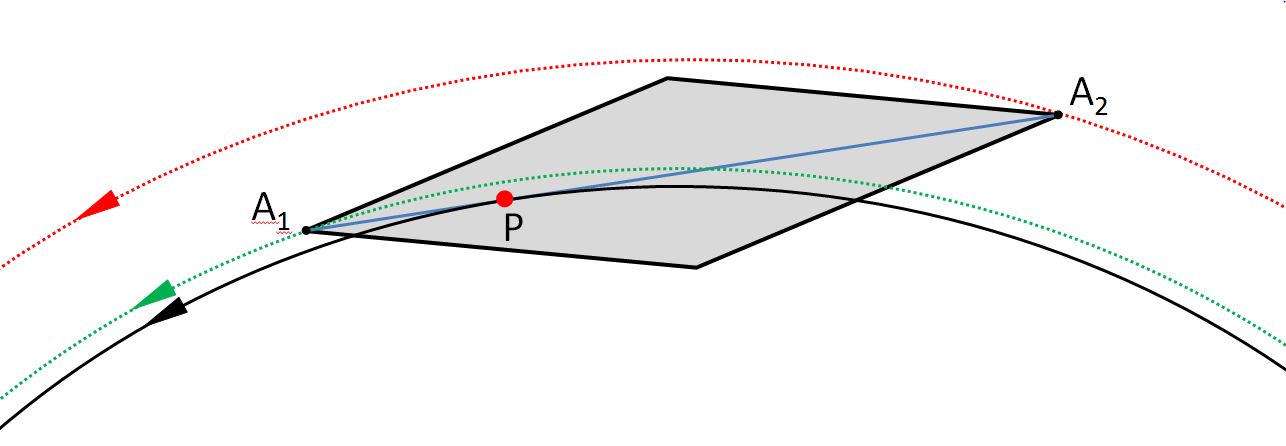
The observed paths are shown in red and green doted lines. If the hypothesis is true, the path of the diatom (except for fluctuations) can be limited to the black trajectory, which the point P passes through. The use of a coordinate pair is sufficient then.
If the two radii of the curvature of the observed trajectories are determined from a short path segment, the distance from P to A₁ can be calculated with elementary geometry. In view of the inaccuracy of the determination of the radii on a short curve segment and the stochastic effect, this simple approach has not proven itself.
It is much more precise to determine P by making an assumption of its position, and then evaluating the angle between the tangent to the trajectory of the hypothetical P and the apical axis along the whole available trajectory. The sum of the squares of the angles between the tangent vector and the apical axis is very suitable for this purpose. The required P minimizes the mean squared deviation (variance) of these angles. By varying the position of the assumed point the minimum is quickly found.
Incidentally it is also possible to use the summed scalar products between tangent vector and apical axis as criterion.
The partly strong stochastic fluctuations prove to be cumbersome. Therefore the curve was smoothed tangentially and transversally by an FIR filter (low-pass).
By means of simulated, artificially disturbed curves, one can check whether the method provides valid results. It has been found that the analysis yields reliable results.
For the specific path curve presented here, the following graph shows the variance of the angles plotted against the position of the assumed point P:
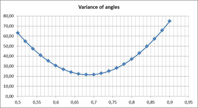
The positions of the trackers are used as a reference for the position of the point P. The value 0 corresponds to the trailing tracker, the value 1 to the leading tracker. At 0.5 the point P lies exactly between the trackers. As the trackers do not sit exactly on the apices, but are slightly shifted inwards, a correction has to be done. On the normed segment A₁A₂ the maximum lies at about 0.64. The point P is located on the side of the apex in the direction of movement, as it is also shown exemplary in the above sketch. As a trajectory of the diatoms, I denote only the path of the point P.
The analysis of other trajectories of the same species often showed similar values. The values for 10 analyzes were between 0.58 and 0.77. Two other species of Navicula yielded somewhat lower values.
As the orientation of the diatoms varies around the direction of the tangent to the trajectory of P, the frequency of the angular deviation can be represented in form of a histogram:
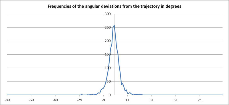
The measured value for P was used here. If the position of P is incorrect, this frequency distribution is not symmetrical to the origin.
The existence of the point P with the described relationship between tangent to the trajectory and orientation of the apical axis is heuristic and should be viewed critically. On the other hand, it has proved its worth in the studied Navicula spp.
In the subsequent analysis the distribution of the velocity (measured μm/second) can be seen:
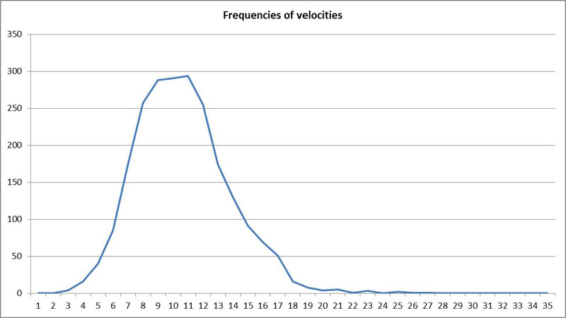
The mean value here is 10.16 μm/s and the standard deviation is 3.07 μm/s. It facilitates the imagination if we relate the velocity of diatoms to their size by measuring in the unit “bodies per second”. In this case the value is about 0.25 bodies per second. The speed can be very different even for the same species. For Navicula the observed range is from a few μm/s to almost 20 μm/s. It turns out that these values strongly depend on environmental influences such as the light field intensity. Some species become mobile only in daylight, others also move during the nighttime.