
")


Size of the diatoms in a chain-like colony I
In this article we will discuss the sequence of diatoms sizes in such a culture and if one can observe them.
| Note: |
A more detailed analysis of the size sequence of diatoms in chain-shaped colonies is given in this publication: Harbich, T. (2021), On the Size Sequence of Diatoms in Clonal Chains. In Diatom Morphogenesis (Diatoms: Biology and Applications) Vadim V. Annenkov (Editor), Richard Gordon (Editor), Joseph Seckbach (Editor), Wiley-Scrivener; First published: 29 October 2021, https://doi.org/10.1002/9781119488170.ch3
The mathematical aspects are treated more formally in the paper than here. As examples for measured sequences, Eunotia sp. is used. Furthermore, a rule of thumb for the loss of synchronicity is derived. |
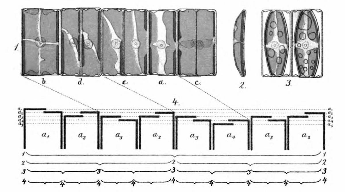
As early as 1871, Pfitzer illustrated the successive reduction in size on the example of a short chain of diatoms of the genus Eunotia (see figure above). Specifically, attempts are being made to determine possible positions of a fragment of such a colony in the theoretical sequence. For this purpose, the sequence of sizes and orientations of the diatoms in a clonal chain must be known first. Ussing et al. (2005) have argued that the generation rule for this sequence can be described by a one-dimensional Lindenmayer model (see Lindenmeyer, A. (1968)). This model has already been successfully used for various species (e.g. cyanobacterium Anabaena catenula).
Both the measurement of the size of diatoms as well as the assignment to the theoretical sequence prove to be no easy task. A closer look at the Lindenmayer system for chains of diatoms makes it possible to successfully analyze an example from nature. This is probably not the case for all species. Furthermore, one cannot assume that a found assignment is unique. In the following, the mathematical basics are explained and the practical challenges described. Then the mathematical method for analysis is presented and demonstrated by an example. So if you want to know more about it, you will find the details below.
Description of the sequence of diatom sizes
Preliminary remark on asexual reproduction
The asexual reproduction of diatoms has already been briefly described in the introduction. Each cell division produces a diatom of the same size and a smaller one. In the following, the possible sizes of the larger valve are indexed by consecutive numbers k, where k = 0 corresponds to the largest possible diatom and kmax to the smallest. Starting from a cell of maximum size (generation 0) there exist in the generation n
![]()
diatoms of the size k (Animation in the introduction shows Pascal’s triangle). The applicability of the formula presumes the synchronicity of the divisions and applies only until the smallest possible cell is reached. If the results for a generation n are normalized to 1, the probability function for the binomial distribution is obtained (probability p = ½). In such an exemplary culture however, there is no probability distribution of the diatoms, but the number of diatoms of a certain size is deterministic. If samples are taken they are following a binomial distribution.
Lindenmayer system
Now the modeling of the colony by a Lindenmayer system is shown. A Lindenmayer system is a triple
D = (A, P, ω) consisting of an alphabet A, replacement rules P (also called productions) and an axiom (start word). The elements of the alphabet are intended to describe the orientation and size of the diatoms in a colony. A colony or a fragment thereof is characterized by a string of characters over the alphabet. The replacement rules P specify how this string changes from generation to generation. A starting condition ω, the so called axiom, determines with which string to start the calculation.
Alphabet A:
Let us imagine the colony as a sequence of characters (a string) written horizontally. The subsequently used notation for the characters of the string has been adopted from Ussing et al. (2005). A diatom whose left valve is larger than its right valve and whose larger valve is given by the size index k is called Lk.
Graphical representation of Lk: ![]()
Correspondingly, a diatom whose right valve is larger than its left valve and whose larger valve is given by the size index k is called Rk.
Graphical representation Rk: ![]()
Lk and Rk are mirror-symmetrical. The alphabet consists of the union of sets { Lk | k = 0, 1, 2, …. kmax } and
{ Rk | k = 0, 1, 2, …. kmax }.
Production rules:
If a diatom that is characterized by the character Lk divides, two diatoms are generated in this arrangement:
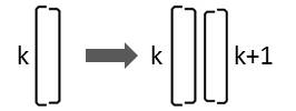
Consequently the following replacement must be carried out:
Lk → Lk Rk+1
If the larger valve of the diatom is on its right side, it is only oriented differently to the observer:
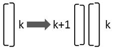
This replacement rule results from mirroring:
Rk → Lk+1 Rk
It is assumed that the cell divisions are synchronous. In the transition from one generation to the next generation, all elements must be replaced according to these rules so that the number of diatoms is doubled. The strings generated correspond to snapshots between the divisions.
With these replacement or production rules the Lindenmayer system is deterministic and context-free and is called a D0L-system.
Axiom:
As an axiom (starting point) I choose a single cell of maximum size corresponding to the status after sexual reproduction. As the orientation of the cell is arbitrary, the axiom can be selected as ω = L0. Ussing et al. (2005) use ω = R0, which leads to mirrored, thus reversed chains. For practical reasons, which will be explained later, I prefer L0. In connection with the properties of the chains produced, their dependence on the axiom will also be discussed.
Beginning with the axiom, the productions are applied iteratively to all elements of the string in parallel. This results in a sequence of strings Gi which describes the colony after the i-th iteration, which is nothing but the i-th generation.
G0 = ω = L0
G1 = L0 R1
G2 = L0 R1 L2 R1
G3 = L0 R1 L2 R1 L2 R3 L2 R1
etc.
In the following, I will term the string that is created after n iterations as "n-th generation".
Observation and challenges
As the MacDonald-Pfitzer rule has often been proved and the description of chain-like colonies is based solely on this rule, a proof of the sequence of sizes should not be difficult at first sight. Nevertheless, I had to realize that this is by no means the case. The following difficulties arise:
- Missing assignment of sizes to size index: When measuring a valve size, there is usually no way of assigning this value to the size index introduced above. In particular, the length of the largest possible valve is not known.
- Too short chains: Even if a fragment consisting of only a few diatoms can be measured well, a match with a theoretical sequence of sizes is only of limited value. It could be due to chance.
- Dead cells in the fragment.
- Small differences in the size of the valves of a diatom: The conception of valves which lie clearly inside one another, may not apply to many diatoms that form chains. The valve sizes appear to differ only by a fraction of their thickness. Natural fluctuations in the size of the valves could also play a role. A sufficiently accurate evaluation of the sequence of sizes of the Melosira colony which has been shown above was not possible to me.
The latter difficulty could possibly be overcome by the use of scanning electron microscopy. Even if all these challenges are mastered, the question remains whether the cell divisions that led to the whole fragment were really synchronized.
In the investigation of the lengths of Eunotia sp. the motility of the diatoms led to further problems. Fragments of several diatoms can separate from the colony. Individual diatoms often migrate away from the ends of the chain and can also detach and move away from the inside of the colony. Such a gap sometimes closes again as a result of expansion through cell division, so that the change remains undetected. The video below left shows several such events in 1500-fold time-lapse. Scenes further apart in time are interrupted by a dark pause. Surprisingly, it even happens that a diatom connects to the end of a chain, as can be seen in the video (1500x time lapse) at the bottom right (near the left edge of the frame). Individual free diatoms settle after some time and form a colony by dividing. It should be mentioned that these observations were made on cultures using the inverted microscope. The illumination (LED) of the microscope replaces daylight. In darkness the movement of the Eunotia comes to rest.
Ussing et al. (2005) discuss the sequence of size on the background of studies on Bacillaria paradoxa, but there is no indication as to whether this principle was observed and whether this was successful.
By chance I found on the internet at http://www.wunderkanone.de/ an excellent picture of a Fragilaria colony, which offers itself at first glance as an examination object. The next picture is shown by courtesy of Eckhard Völcker (see http://www.penard.de/):
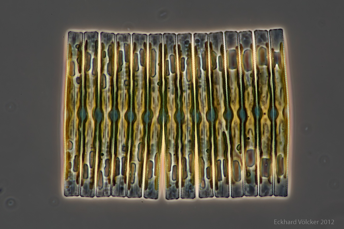
Each of the diatoms shows significant differences in size between their valves, which is evident in the irregular upper and lower edges. The fragment contains 14 diatoms. A quite advanced breaking point is visible between the 6th and 7th diatoms from the left.
An easy possibility to assign the sizes of the diatoms to a size index is not given. In order to be able to verify the agreement with the theory, however, it is useful to study the properties of this Lindenmayer system in more detail. Therefore, I return to the theory.
Properties of the Lindenmayer system
Two simple rules of this D0L-system prove to be particularly important:
Symmetry:
A chain of diatoms is characterized by a string with characters of the alphabet Lk and Rk with K = 0 .. kmax. If you look at it mirrored, so that the right and left are interchanged, the corresponding string must be reversed. In addition, each L must be replaced by an R and each R by an L so that the orientation of each diatom is also changed. The operator of the reflection is denoted by S. The production rules (operator P) are invariant under reflection by construction, so that P∘S = S∘P holds. It is irrelevant whether you first perform a mirroring and then an iteration or vice versa. This simply means that the growth of a chain-like colony does not depend on the direction from which it is viewed.
Change of size index:
It is helpful to consider the strings generated by iterations of the production rules of the described D0L-system as a function of the starting point. According to the production rules, a diatom of size k produces in the case of asexual reproduction a diatom of the same size k and a smaller one with size index k + 1. If one starts with the axiom Lk instead of L0 where k> 0, then in the first generation according to the Production rules, all size indices are increased by k. This is also true in the second and subsequent generations.
If therefore the development of two colonies is observed where each colony starts with a single diatom of different size, similar size patterns are produced, but the size indices in one chain is shifted by a constant value relative to the other chain. If the differences of the size indices of successive diatoms are calculated, these differences are identical for both chains. This is the basic idea when answering the question of how far a fragment of a colony can be assigned to a theoretical sequence without knowledge of the mapping of size indices to absolute lengths.
Alternative formulation
These two rules make it possible to derive an alternative formulation for the calculation of generations. In the following figure, the first 5 generations are arranged one below the other starting from the axiom. The numbers denote the size indices. In order to simplify the notation, the orientation of the diatoms is marked by font colors. Black characters stand for "L" and red for "R".
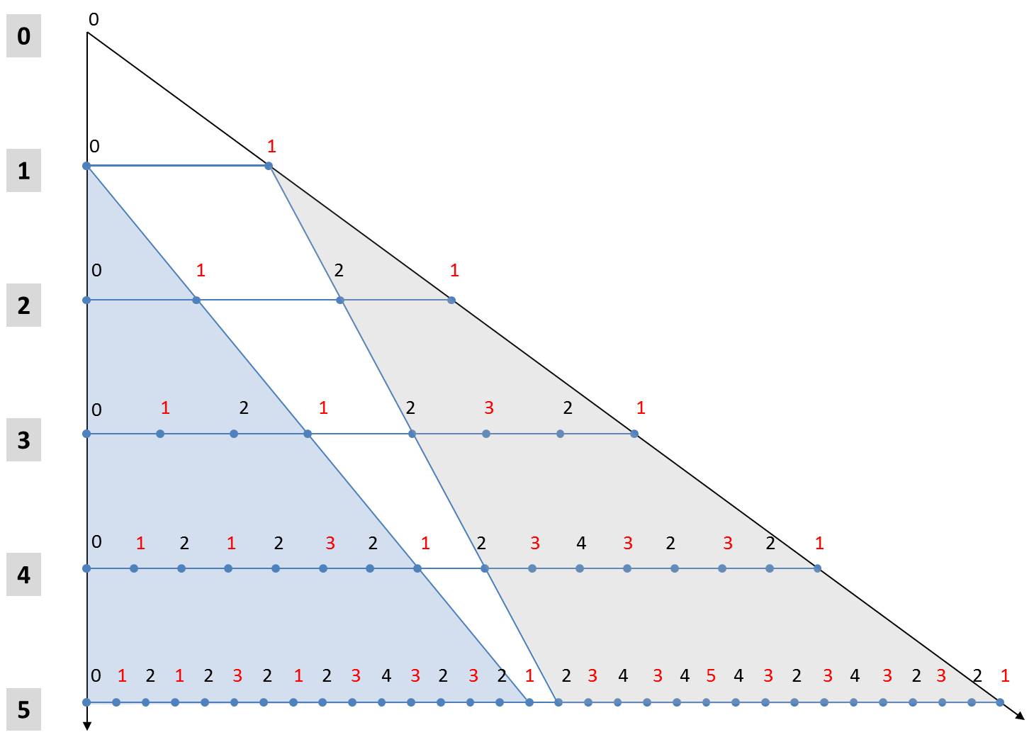
The fifth generation to Axioms L0 can be seen with its 25 elements in the last row. The light blue triangle shows that its first 24 elements are equal to the 4th generation with respect to the same axiom L0. The same applies obviously for all other iterations beginning with the first iteration. In each case, the first half of the n-th generation is identical to the (n-1)-th generation to the same initial value L0.
A little more complicated is the rule for the 2n-1 elements of the second half of the generation. From the gray triangle it can be seen that the second half of the n-th generation is the (n-1)-th generation with respect to the initial state R1. The two above-mentioned rules can be used to determine the associated characters. All elements of the n-1-th generation belonging to the initial value R1 are higher by the value 1 compared to a start with the hypothetical value R0. In addition, they are mirrored in comparison to a generation which originates from the starting element L1. The values of the second half of the n-th generation can thus be obtained from the (n-1)-th generation belonging to the axiom L0 by mirroring (exchanging "L" and "R" and reversing the order) and incrementing all size indices. The (n-1)-th generation is identical to the first half of the n-th generation.
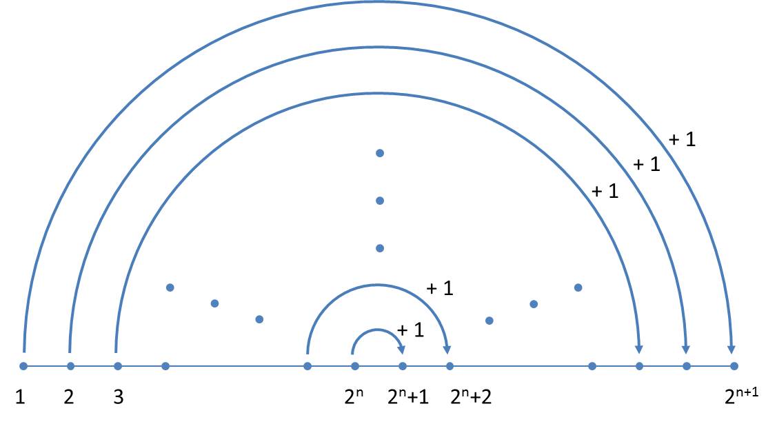
This representation provides a simple scheme to determine generations. If a generation is available, the next generation can be written down by the following scheme without explicitly using the replacement rules:
- The present generation is the first half of the next generation.
- The second half of the next generation is obtained by mirroring (exchange of "L" and "R" and reversing the order) of the present generation with simultaneous increase of all size indices by the value 1.
In each generation the orientations (a note to the proof is given below) are alternating, so that one can limit yourself to the size indices. The simplified scheme is illustrated below:
Now it becomes clear why, in contrast to Ussing et al. (2005), a mirrored axiom is used. As we write from the left to the right, the next generation can always be completed at the end.
Denoting the size indices of the n-th generation with ain, where i takes the values 1 … 2n, the generation rule reads as follows:
![]()
The initial value corresponding to the selected axiom is a10 = 0. A formal mathematical proof is given in the publication cited above, "On the size sequence of diatoms in clonal chains".
If one knows the absolute indices of the size of a found fragment of a colony, one can search for the generation in which this or the mirrored pattern appears for the first time. All subsequent generations contain the same pattern, so that there can be no unique assignment to one generation.
This formulation not only allows the rapid manual calculation of the generations, but also provides some mathematical insights immediately. For example there is no periodicity because of incrementing.
The repeated duplication with mirroring produces a self-similar fractal structure. The following diagrams show the size indices for the 8th to 11th generation. Each diagram forms the first half of the subsequent diagram..
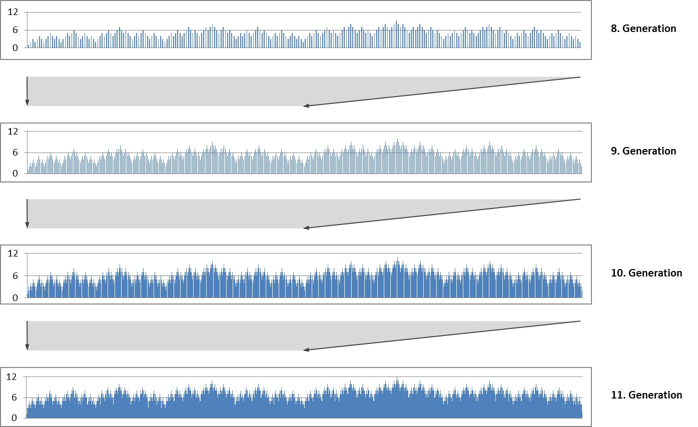
Self-similarity and fractal structure are not surprising because they are typical for Lindenmayer systems.
When one increments the next maximum size index results from the previous maximum size index. In accordance with Pascal’s triangle, the maximum value in the nth generation is n. For its position in the string it is easy to formulate a relationship. In the limit n → ∞ the position converges to 2/3 of the length of the string.
More important for our purposes are the following statements, which apply from the 1st generation for each further generation:
- The orientations of the diatoms alternate.
- The differences of successive size indices (size index of an element - size index of its predecessor) can only take the values +1 or -1.
Both assertions can be proved in a few lines by complete induction. The first statement can alternatively be derived immediately from the replacement rules. As base case the first generation is used. For the inductive step the upper half of the n + 1-th generation and the position where the lower and upper halves border each other have to be considered. The first half of the n-th generation need not to be considered more closely because it is identical to the (n-1) generation (induction hypothesis). The second statement turns out to be useful for the characterization of a fragment.
The difference sequence of neighbouring elements in the nth generation contains n-1 elements. They are independent of the size index used in the axiom. A simple schema can also be given for the generation of the sequence of differences which follows immediately from the schema for the size indices. In the transition to the next generation, one firstly appends the number 1 to the existing generation and then reflects the previous generation whereby all values have to be inverted:
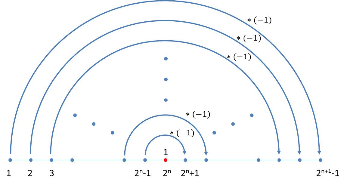
If the differences between the size indices of the n-th generation are denoted by din, where i takes the values 1 … 2n – 1, the iteration formula reads:
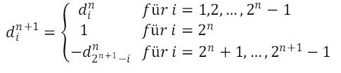
As the iteration requires at least one difference we start with the initial value d11= 1.
Analysis of the lengths of the fragment
It is time to return to the analysis of the above shown fragment of a Fragilaria colony. First of all, one can see that the orientation of the diatoms is alternating in accordance with the theory.
 |
 |
In the picture on the left you see side by side narrow stripes which were cut out of the overall image showing the longer valve of each diatom (click to enlarge). Although this is an example where the sizes of diatoms can be differentiated their differences are relatively small. On average, length differences between adjacent diatoms are about 0.6% of their mean length. The absolute values of the differences in length between neighboring diatoms are not constant because of the limited resolution and presumably also of natural fluctuations. Small adjustments of the marks have a very strong effect due to these very small differences.
The bar chart below shows the absolute values of the differences in length (in percent of the mean cell length) of adjacent diatoms is therefore to be considered critically.
The biggest problem is the 10th value, which deviates extremely from the other values. Otherwise, there are no differences in length, which differ from the others by a factor of 2 or 3. If one considers the D0L-system in spite of this strong deviating value for plausible, the sizes of the diatoms can be analyzed except for an additive constant. One considers only the feature of whether a diatom is longer or shorter than its predecessor. If it is longer, the difference is -1, otherwise 1. The 10th value (-1) is to be regarded as uncertain because of the anomaly mentioned. These differences are shown in the figure above. Since, as mentioned several times, an assignment to the absolute magnitude index is missing, I consider the sequence -1 1 1 -1 -1 -1 1 1 -1 -1 1 -1 -1 as a "fingerprint" of the fragment of the colony.
Now one can check whether the fingerprint can be found in a sufficiently long sequence of differences. With a length of the fragment of 14 diatoms, i.e. 13 length differences, it can occur at the earliest in the 4th generation. It is found mirrored and inverted in this generation (1 1 -1 1 1 -1 -1 1 1 1 -1 -1 1). Here the sequence of differences of the 4th generation can be seen, whereby the mirrored inverted "fingerprint" of the fragment is highlighted by red color:
1 1 -1 1 1 -1 -1 1 1 1 -1 -1 1 -1 -1
In the sequence of sizes belonging to the axiom L0 the fragment can be placed accordingly:
0 1 2 1 2 3 2 1 2 3 4 3 2 3 2 1
Here the size index of the first diatom from the left is 0, the largest occurring index is 4. The correspondence between observed and calculated patterns is convincing and proves again the MacDonald-Pfitzer rule. Above all, it demonstrates the practical usability of the D0L-system.
Number of pattern matches
As a result of self-similarity, the fingerprint of the diatom fragment can be found additionally in the next generation mirrored and inverted. For the fragment there are two places with matching patterns. To fit in the second location, it must be mirrored. With each generation the sites with matching patterns are doubled. If the pattern of the fingerprint appears for the first time in the generation m, then it is found in the generation j with j ≥ m exactly 2j-m times. The unknown absolute assignment of the length to a size index thus leads to further possibilities of placing a fragment into the theoretical size sequence.
LINDENMAYER, A. (1968a). Mathematical models for cellular interactions, in development
I. Filaments with one-sided inputs. Journal of Theoretical Biology, 18, 290-299
Pfitzer, E. (1871) Untersuchungen über Bau und Entwicklung der Bacillariaceen (Diatomeen).
Botanische Abhandlungen 2, 1–189.
USSING, A.P., GORDON, R., ECTOR, L., BUCZKO´ , K., DESNITSKIY, A.G. & VANLANDINGHAM, S.L. (2005). The colonial diatom ‘‘Bacillaria paradoxa’’: chaotic gliding motility, Lindemeyer Model of colonial morphogenesis, and bibliography, with translation of O.F. Müller (1783), “About a peculiar being in the beach-water”. Diatom Monographs, Vol. 5. Koeltz, Koenigstein, Germany.